- Download
- Welcome to SOFiA
- Who is behind SOFiA
- Feature overview
- System overview
- Function reference
- readVSAdata
- mergeArrayData
- F/D/T
- gauss
- lebedev
- S/W/G
- S/T/C
- W/G/C
- S/F/E
- M/F
- R/F/I
- P/D/C
- I/T/C
- makeMTX
- makeIR
- visual3D
- Coordinate System
- Application Examples
- Example 1
- Example 2
- Example 3
- Example 4
- Example 5
- Example 6
- Example 7
- Example 8
- Array Datasets
- VariSphear system
- Groups and Mailinglists
- Contact and Support
- How to Reference
|
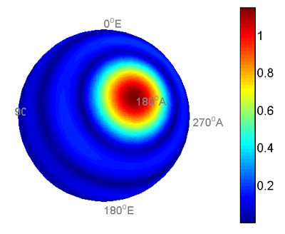
SOFiA application example 3
This example shows a real "plane wave" produced by a speaker system in the anechoic chamber. The wave impinges to the backside of the array (180°AZ, 90°EL). The array is configured as an open sphere array with a Microtech Gefell M900 large diaphragm cardioid transducer sampling on a Lebedev 86P grid at a radius of r=0.25m.
File(s)
Run `sofiaAE3.m`.
Locate the folder `EXAMPLE4_CardioidMic` containing the required array data.
Output
Code
/*
% SOFiA example 3: A measured plane wave from AZ180°, EL90° in the anechoic chamber using a cardioid mic.
% SOFiA Version : R11-1220
% Array Dataset : R11-1018
clear all
clc
% Read VariSphear dataset
% !!! LOCATE THE FOLDER: "EXAMPLE4_CardioidMic"
timeData = sofia_readVSAdata();
% Transform time domain data to frequency domain and generate kr-vector
[fftData, kr, f] = sofia_fdt(timeData);
|
% Spatial Fourier Transform
Nsft = 5;
Pnm = sofia_stc(Nsft, fftData, timeData.quadratureGrid);
% Radial Filters for a rigid sphere array
Nrf = Nsft; % radial filter order
maxAmp = 10; % Maximum modal amplification in [dB]
ac = 1; % Array configuration: 2 = Rigid Sphere
dn = sofia_mf(Nrf, kr, ac, maxAmp); % radial filters
dn = sofia_rfi(dn); % radial filter improvement
|
% Make MTX
Nmtx = Nsft;
krIndex = 600; % Here we select the kr-bin (Frequency) to display.
mtxData = sofia_makeMTX(Nmtx, Pnm, dn, krIndex);
% Plot the response
figure(1)
clf();
sofia_visual3D(mtxData, 0);
view(90, 0)
disp(' ');
disp('The plot shows the response at a frequency of ',num2str(round(10*f(krIndex))/10),'Hz');
|
*/ |
|
|

